Benchmarking
GSWHC-B Getting Started with HPC Clusters \(\rightarrow\) PE3-B Benchmarking
Relevant for: Tester, Builder, and Developer
Description:
You will learn to assess speedups and efficiencies as the key measures for benchmarks of a parallel program (basic level) (see also K2.1-B Performance Frontiers)
You will learn to differentiate between strong and weak scaling (basic level)
You will learn to benchmark the runtime behavior of parallel programs, performing controlled experiments by providing varying HPC resources (e.g. 1, 2, 4, 8, … cores on shared memory systems or 1, 2, 4, 8, … nodes on distributed systems for the benchmarks) (basic level)
You will learn about the performance impact of certain features of current CPU architectures (temperature and dynamic CPU frequencies) (basic level)
This skill requires the following sub-skill
- K2.1-B Performance Frontiers (\(\leftarrow\) K2-B Performance Modeling)
Level: basic
Motivation
Benchmarking means the comparative analysis of measurement results of certain program properties for the performance determination of hard- or software. The measurement results, primarily those of the program runtimes, are determined by controlled experiments.
Such a controlled experiment is named a benchmark, but the term is also used – apparent from the context – for the program that is, or set of programs that are used for benchmarking.
For HPC users measuring the performance behavior of the parallel program(s) they use is of primary importance in order to make optimal use of HPC hardware. Hence this is the focus of this learning unit.
Before benchmarking is explained in more detail, standard benchmarks, like Linpack, shall briefly be mentioned here for the sake of completeness.
Benchmarking hardware
The Linpack benchmark is used, for example, to build the TOP 500 list of the currently fastest supercomputers, which is updated twice a year. The computer’s floating-point rate of execution is measured by running a program that solves a dense system of linear equations. Beside the floating point operations per second (FLOPS), the Top 500 list contains a number of additional details of the different supercomputers, like CPU architectures, power consumption, number of cores, etc. Such information shows current trends in HPC and is of great interest for computing centers with view to the procurement of next generation cluster system.
It is also common practice to execute a mixture of different parallel programs to get impressions of the total performance of a cluster system under conditions simulating practical use.
Benchmarking software
For HPC users, however, synthetic tests to benchmark HPC cluster hardware (like the Linpack benchmark) are of less importance. For them, the emphasis lies on the determination of speedups and efficiencies of the parallel program they want to use with regard to varying the number of cores (or cluster nodes) for the measurements.
This kind of benchmarking is very essential in the HPC environment and can be applied to a variety of issues:
What is the scalability of my program?
How many cluster nodes can be maximally used, before the efficiency drops to values which are unacceptable?
How does the same program perform in different cluster environments?
Benchmarking is also a basis for dealing with questions emerging from tuning, e.g.:
What is the appropriate task size (big vs. small) that may have a positive performance impact on my program?
Is the use of hyper-threading technology advantageous?
What is the best mapping of processes to nodes, pinning of processes/threads to CPUs or cores, and setting memory affinities to NUMA nodes in order to speed up a parallel program?
What is the best compiler selection for my program (GCC, Intel, PGI, …), in combination with the most suitable MPI environment (Open MPI, Intel MPI, …)?
What is the best compiler generation/version for my program?
What are the best compiler options regarding for example the optimization level
-O2,-O3, …, for building the executable program?Is the use of PGO (Profile Guided Optimization) or other high level optimization, e.g. using IPA/IPO (Inter-Procedural Analyzer/Inter-Procedural Optimizer), helpful?
What is the performance behavior after a (parallel) algorithm has been improved, i.e. to what extend are speedup, efficiency, and scalability improved?
If the focus is on performance improvements, the user should also feel motivated to benchmark the program after any change of the environment, the configuration, or the program itself.
Benchmarking the runtime behavior of parallel programs
For benchmarking a parallel program at the basic level it is essential to measure its runtimes in dependence of the HPC resources provided (e.g. 1, 2, 4, 8, 16, 32, 64, … cluster nodes) in a series of experiments.
For a parallel program that uses a single cluster node only, as a typical OpenMP program, controlled experiments to measure the execution time are performed in a similar way providing an increasing number of cores (e.g. 1, 2, 4, 8, 16, …) in this case.
The parallel efficiency \(E\) is the ratio of the speedup \(S\) achieved in an experiment to the number of cluster \(nodes\) or \(cores\), respectively, used in the experiment:
\[ E_{nodes} = \frac{S_{nodes}}{nodes} \]
or
\[ E_{cores} = \frac{S_{cores}}{cores}. \]
Below, two Tables with hypothetical benchmark results are given as examples for measuring the runtimes of a parallel program to calculate \(\pi\) with the same vast number of decimal places in each experiment:
| Program | Runtime [s] | Cluster Nodes | Total Cores | Speedup | Efficiency |
|---|---|---|---|---|---|
| calc-pi-MPI | 180.5 | 1 | 16 | 1.00 | 100% |
| calc-pi-MPI | 92.1 | 2 | 32 | 1.96 | 98% |
| calc-pi-MPI | 47.5 | 4 | 64 | 3.80 | 95% |
| calc-pi-MPI | 25.1 | 8 | 128 | 7.19 | 90% |
| Program | Runtime [s] | Total Cores | Speedup | Efficiency |
|---|---|---|---|---|
| calc-pi-OpenMP | 2800.0 | 1 | 1.00 | 100% |
| calc-pi-OpenMP | 1414.1 | 2 | 1.98 | 99% |
| calc-pi-OpenMP | 707.1 | 4 | 3.96 | 99% |
| calc-pi-OpenMP | 360.8 | 8 | 7.76 | 97% |
How can runtimes be measured?
For the total runtime of programs started interactively, the answer is simple: the time command will do the trick.
Note that many shells (including bash) have a built-in time command, which may offer less features than the globally installed stand-alone program. For MPI programs the shell built-in gives enough relevant information:
time mpirun ... my-mpi-appFor a sequential or an OpenMP program /usr/bin/time gives more interesting information than time in addition:
    export OMP_NUM_THREADS=...
    /usr/bin/time my-openmp-app
Scaling
The scalability of a program is considered to be good when the efficiency remains high when the number of processors is steadily increased.
As work is distributed among more and more processes the overheads for synchronization (e.g. waiting for partial results of other processes) and communication (e.g. distributing partial data or tasks to other processes and collecting partial results from them) are also increasingly growing. Eventually, this will lead to a reduced performance of the program and the efficiency will drop.
Typically, there exists a dependency on the problem size, e.g. on the size of a matrix, to be processed with a parallel algorithm.
Two types of scalability can be distinguished that deal with the question of how many nodes (or cores) can be reasonably used to further reduce the time to solution to solve a problem. It is required for:
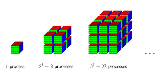
Weak scaling, that the problem size increases proportional to the number of parallel processes.
In other words, weak scaling answers the question: How big may the problems be that I can solve?Strong scaling, that the problem size remains the same for an increasing number of processes.
In other words, strong scaling answers the question: How fast can I solve a problem of a given size?
A typical use case for weak scaling is to predict the performance for using very many processes.
For illustration scaling plots are shown below. These were obtained from benchmarking conjugate gradient solvers in simulations of lattice gauge theories. The main properties of these kinds of calculations are:
The problems are 4-dimensional. The data access pattern is given by a 9-point stencil.
Communication patterns are halo boundary exchange and global sums.
Weak scaling
For weak scaling the number of processors \(n\) is increased and the domain size \({data}\) (i.e. the size of the problem) per process is kept constant, i.e. total domain size \({data_{n} \propto {n}}\).
This typically leads to the following observations:
Communication overhead of boundary exchange increases at low process counts
Sustained performance per process is roughly constant at high process counts
Weak scaling plot example
In the plot below performance per core is plotted over the number of cores used. Typical weak scaling behaviour can be seen: performance per process decreases when more cores are used and then flattens out at some point.
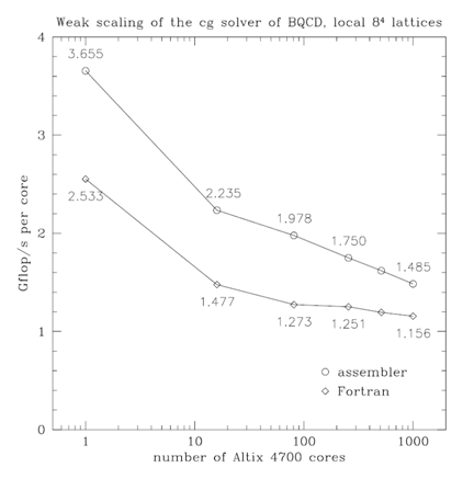
If performance figures are not available execution time can be plotted. Execution time is expected to increase and then flatten out.
A logarithmic \(x\)-scale is better suited if the number of processes varies over orders of magnitudes
Strong Scaling
For strong scaling the number of processors \(n\) is increased and the total domain size \({data}\) (i.e. the total size of the problem) is kept constant.
This typically leads to the following observation:
- domain size per process decreases,
- communication overhead increases,
- sustained performance per process decreases.
The motivation for studying strong scaling is to determine an optimal number of processes to use.
The question whether an efficiency may be considered to be acceptable depends on context, e.g. the algorithm a program is based on, and on boundary organizational or “political” conditions: the more important it is to reduce the time to solution, the lower a still acceptable efficiency will be.
Normally, it will obviously be harder to achieve acceptable efficiencies for strong scaling conditions than for weak scaling conditions when the number of processors is steadily increased.
Strong scaling plot examples
A classic strong scaling plot shows speedup over the number of processes. A reference point needs to be defined where the speedup is 1. Originally, a single process was chosen where the (parallel) program is executed sequentially. Nowadays, a single node is a natural reference point. Other points can be chosen, e.g. a rack.
Typically, linear scaling is indicated in a strong scaling plot for comparison. Double logarithmic plots are advantageous because orders of magnitudes can be better resolved (linear scaling is still represented by a straight line in double logarithmic plots).
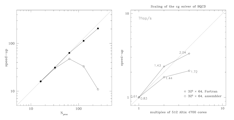
In the figure above two scaling plots are shown. The plot on the left hand side shows bad scaling (open circles) of an early parallel program in which the global sum was implemented in a naive way (the computational effort was proportional to the number of processes used) and good scaling (filled circles) that was achieved after implementing an improved version of the global sum (using a binary tree algorithm, which has only logarithmic complexity). In this case the reason for bad scaling is a naive algorithm. Two points should be remembered:
- Even the bad implementation could by used with up to 64 processes.
- The speedup curve of any parallel program will bend down if too many processes are used.
The plot on the right hand side shows speedup curves for two different implementations of the solver of the BQCD program. The Fortran implementation (diamonds) displays a superlinear speedup from 512 to 1024 cores. The assembler implementation (circles) is faster on 512 cores. On 1024 cores both implementations run at about the same speed. On 2048 cores the speedup is unacceptably low in both cases (the efficiency compared with running on 1024 cores is 71% for the Fortran and 60% for assembler implementation). The plot was chosen in order to explain how to decide on the number of processes that can reasonably be used.
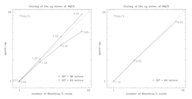
The next plot, above, shows scaling results for two different problem sizes obtained with a Fortran implementation (left hand side) and an assembler implementation (right hand side). Remarkable is that
- the larger problem (diamonds) displays superlinear speedup from 1 rack (2048 cores) up to 8 racks (16384 cores),
- the assembler implementation can improve performance on the smaller problem (circles) considerably and scales almost linearly (this occurs because communication and computation overlap in the assembler implementation).
While these observations are specific to the problem, important general observations can be made as well:
- Plotting speedup can be misleading when only scaling curves are compared, i.e. scaling can look better, while performance is worse. One has to look at performance, too.
- Generally, slow programs scale better.
In instead of speedup one can directly plot performance. For demonstration this was done with the data from the figure above on the left hand side of the plot shown below. In such a plot one can directly compare scaling and performance. Because there is no reference point there is no single reference line for linear performance (through any point such a line could be drawn). The plot contains three lines that indicate linear scaling to guide the eye.
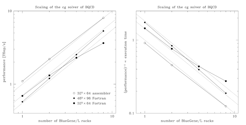
If performance figures are not available one can make the same kind of plot from execution times. This is shown in the plot on the right hand side in the figure above. (In this case just the inverse of performance data was plotted, which is inverse proportional to performance.) In general, one has to normalize times, e.g. plot the time per iteration and mesh point.
Further benchmark opportunities
Some possible application areas of benchmarking have already been mentioned in connection with tuning ideas in the motivation section. Benchmarking can be used for example to determine the most suitable compiler (GCC, Intel, PGI, …) and MPI environment (Open MPI, Intel MPI, …) for building a program that is as fast as possible. It can also be observed now and then, that for some reason a predecessor version of a compiler might create code that is faster than the code created with the current version. This might indicate that the program has to be adopted to the current compiler version so that fast (or even faster) executable code is created again.
To take another example already mentioned in the motivation section, benchmarking can also be used to answer the question if there is a positive trade-off to be expected when performing the typical two steps of the Profile Guided Optimization (PGO) cycle consisting of
Step 1: running initially the instrumented (and therefore relatively slow) version of the program providing representative input data to collect information about which branches are typically taken and other typical program behavior,
Step 2: recompiling with this information to build a faster program.
For some algorithms and a given constant problem size there might exist an inverse proportional relationship between the main memory provided for the parallel program and the execution time, e.g. when large hash tables can be used for caching partial results that would otherwise have to be recalculated (multiple times) on demand, to give just one example. In this case it may be beneficial for the user to choose a partition (or batch queue, respectively) of a given cluster that offers him a smaller number of bigger nodes (i.e. nodes with a larger amount of main memory) when compared with other partitions that could be chosen. Appropriate benchmarks can be used to examine if it is advantageous to use the nodes with the larger amount of main memory.
Besides performing benchmarks depending essentially on the computing power of a cluster system it might also be interesting to benchmark the network bandwidth (e.g. InfiniBand vs. Ethernet) or the I/O performance of the file system of cluster systems. This is interesting in particular if the user can choose between such possibilities, e.g. if different cluster systems are available to submit batch jobs to. Within the same cluster it may furthermore be interesting to see which positive impact choosing the adequate file system might have on reducing the runtime, e.g. using a fast SSD (Solid State Disk) instead of the parallel file system for locally storing temporary data.
Pitfalls
Several topics are listed below which should be considered carefully in order to avoid typical pitfalls.
Break-even considerations regarding the benchmark effort
It follows from the foregoing that benchmarking, especially with regard to determining the scalability of a parallel program, is important.
However, benchmarking also represents a certain effort, namely
for providing the HPC resources explicitly used for that purpose,
and human time for (manually) performing the experiments, collecting and interpreting the results.
Test input data representing a comparatively small problem size can often be helpful to assess reasonably accurate the performance behavior for larger problem sizes, without incurring inappropriately high CPU time usages (also see explanations of weak and strong scaling above).
Depending on the purpose, varying the provided HPC resources for benchmarking can be performed in larger steps, so that for example 1, 4, 16, 64, … cluster nodes are used for the series of experiments. This way the HPC resource usage as well as the (manual) effort to manage the experiments can be greatly reduced.
Break-even considerations should be kept in mind, but anyway it can be assumed that there will usually be a positive trade-off performing benchmarks in an appropriate manner. This is particularly true in connection with tuning, for which benchmarking is the basis.
Presenting fair speedups
For the determination of speedups the parallel program executed on a single core is often considered as sequential version of an algorithm. The runtime measured on a single core is then used as numerator \(T_1\) for calculations like:
\[ S = \frac{T_1}{T_{parallel}} \]
A parallel program might scale pretty well under these conditions. Therefore it is important to be aware of the best known sequential algorithm for such comparisons in order to get fair speedup results (especially when it is planned to publish the results).
Special features of current CPU architectures
The CPU clock rates of a typical multi-core cluster node supporting features like turbo boost may vary depending on the CPU usage. At low CPU load, when for example only a single core is used, the clock rate of this core is typically considerably higher than the clock rate at times when several cores are fully utilized. If many cores are fully utilized over a period of time, the clock rates of the cores will be usually reduced over time to avoid a rise in CPU temperature, which is heavily affected by the clock rates.
The runtime of benchmarks should therefore not be chosen too short, in order to achieve stable CPU clock rates at first. This also has the advantage that possible overheads in the initialization phase, for example for reading extensive input data using just a single core, or in the de-initialization phase, for example for writing final results to a file, again using just a single core, only have a relatively small impact on the runtime.
A meaningful minimum runtime of course depends on the specific parallel program that is to be benchmarked. As a rule of thumb the runtime should be at least a few minutes.
The hyper-threading technology is a further peculiarity of current multi-core CPU architectures. With hyper-threading enabled, each physical core of the CPU can also be used as two logical hyper-threaded cores, each – simply put – just over half as fast as a physical core. Using two hyper-threaded cores mainly improves exploiting functional subunits of the CPU, so both hyper-threaded cores have slightly more computing power than their corresponding physical core (however, depending on the scalability of a program this does in no way imply a positive trade-off for using hyper-threading). If one core of a hyper-threaded core pair is idle, the other core can run at the full speed of a physical core. This already hints that hyper-threading may add some complexity to benchmarking.
Provided that all hyper-threads of all cluster nodes are permanently fully utilized by the parallel program, the runtimes measured in a series of benchmark experiments are comparable with each other very well.
The same applies if hyper-threading is not really used, i.e. if on a node with \(h\) hyper-threaded cores no more than \(h/2\) cores are utilized by the parallel program. In this case all cores can run at the full speed of a physical core.
It will be difficult to determine the scalability of a program, if a number of cores is used for the parallel program for which some hyper-threads are running at the full speed of a physical core and some hyper-threads are running only at about the half speed, i.e. if the number \(n\) of used cores is in the range \(h/2 < n < h\). In such a mixture of core usage it will be hard to assess the speedups achieved in relation to the cores used by calculating efficiencies via \(E_{cores} = \frac{S_{cores}}{cores}\).
Shared resources
It lies in the nature of benchmarking that cluster nodes of the same type should be made exclusively available to the user for benchmark experiments. This avoids the influence of parallel programs from other users – running otherwise possibly on the same nodes at the same time – on the result, i.e. on measuring the execution time as precisely as possible.
In an ideal case, benchmarks are performed (after program changes, for example) even on the same set of nodes they were performed initially, in order to avoid any side effects that might be introduced by using (slightly) different cluster hardware. Such side effects can be caused for instance by manufacturing tolerances of cluster nodes, or differences regarding the interconnection network between nodes.
But even under ideal conditions using the same set of nodes to perform all benchmarks, the program has generally to share some HPC resources with other programs running on the cluster at the same time. These resources include in particular network bandwidth for interprocess communication and I/O bandwidth for accessing a global parallel file system.
In the context of benchmarking, users should be aware of such effects. If they seem actually significant, one idea to alleviate the problem would be to repeat each benchmark several times for calculating averages, or to use the median to avoid the influence of outliers, for example.
Shared nodes
Compute centers often also make shared nodes explicitly available for a cluster system via an appropriate batch queue, or partition, respectively, in which several users may share the cores of the nodes. When the user is only interested in the result of a program, that is usually not much of a problem and it especially enables the compute center to make better use of the expensive HPC resources that would typically be more idling otherwise.
As long as only different cores on the same node are used at any point in time by two or more programs of different users, benchmark results may still be meaningful. If the same cores are potentially shared at times on a node by different programs, the value of the benchmark results may be significantly reduced or even made useless.
Reproducibility
Nowadays, it is increasingly required that scientific results from numerical programs are reproducible, so that they can be verified by external parties.
For parallel programs reproducibility is also important for benchmarking. If the execution of a program depends for example on a randomized component (as used for Monte Carlo algorithms), the random number generator needs to be made deterministic in order to ensure the reproducibility of repeated runs of a program. (Random number generators or, strictly speaking, pseudo random number generators, are typically initialized in a fashion (called seeding) that the sequence of the random numbers generated remains the same every time the program is started.)
However, there are parallel algorithms which may produce non deterministic results, due to inherent effects of concurrency. A variety of parallel tree-search algorithms could serve as a good example. Without going into detail, many tree-search algorithms typically cut-off parts of the search tree during the search. Depending on when branches of the tree are cut off by a search process and how this information is exchanged between all parallel searching processes, usually different parts of the tree are redundantly searched each time the program is restarted. This in turn may lead to different (but generally equivalent) search results and also to strongly differing runtimes of repeated runs.
In the context of benchmarking users should be aware of the existence of parallel algorithms with a non-deterministic behavior (event-driven simulations, for example). One way to alleviate the problem would be to repeat each benchmark several times for calculating averages, another would be to use the median to avoid the influence of outliers.