Performance Frontiers
GSWHC-B Getting Started with HPC Clusters \(\rightarrow\) K2-B Performance Modeling \(\rightarrow\) K2.1-B Performance Frontiers
Relevant for: Tester, Builder, and Developer
Description:
You will learn about FLOPS (floating point operations per second) which is the key measurement unit for the performance of HPC systems, and its pitfalls (basic level)
You will learn about Moore’s law and its significance for performance frontiers in modern HPC (basic level) (background topic)
You will learn about the definitions for key terms: speedup, efficiency, and scalability (basic level)
You will learn about Amdahl’s law and its significance for performance frontiers in modern HPC (basic level)
This skill requires no sub-skills
Level: basic
Floating Point Operations per Second (FLOPS)
A key measure for the performance of HPC systems are so-called floating point operations per second (FLOPS or Flop/s), which are in the order of several PetaFLOPS for the top HPC systems of 2017. One PetaFLOPS (PFLOPS) corresponds to 10\(^{15}\) FLOPS or 10\(^{3}\) TeraFlops (TFLOPS), respectively. In comparison, a stand-alone computer, like a powerful PC, achieves a peak performance of about 1 TeraFLOPS.
This measurement is generally used in two distinct ways:
To measure the computing power of a computer.
In the context of HPC systems, such measurements are collected in the TOP 500 list. This list, which is updated twice per year, lists 500 supercomputers ranked by the FLOPS they achieve in the Linpack benchmark. Because this list also contains a number of additional details of the different machines, like CPU architectures, power consumption, node count, OS, etc., it is a valuable resource to spot trends in the field of high performance computing.
To measure the performance of applications.
Modern CPUs provide the feature of counting every floating point operation that they execute. This can be used to obtain the FLOPS that an application actually uses, and to compare it to its peak performance (the FLOPS that the machine is theoretically able to deliver). The idea is to use this FLOP utilization to assess how well-optimized the application code is.
Pitfalls
While the measurement FLOPS is frequently used to gauge the computing power of a system and of applications, it is also a disputed measurement. Its connection to actual application performance is too loose. For instance, many of the top systems on the TOP 500 list use GPUs to achieve their immense FLOPS, yet many scientific codes perform better on pure CPU based systems.
So, this is a list of the most important pitfalls of using FLOPS to assess computing power:
Many scientific applications are memory bound, not CPU bound.
The arithmetic-logical units that perform the computations are but one of the resources within a CPU. Other resources are important as well, such as caches, instruction decoder slots, and memory buses. If there is not enough computation to be done for each value that is fetched from memory / stored to memory, the memory buses will saturate and become the bottleneck of the application.
Typical offenders of this include computing the dot product of two long vectors: This will repeatedly load two values (2x8 = 16 bytes) from memory, and then execute a single fused-multiply-and-add operation (fmadd). With vectorization, four of these operations can be performed in a single instruction, but require fetching 4x16 = 64 bytes to work on. A DDR4-3200 memory module can deliver 25.6 GByte/s, which is just enough input data for 400 million arithmetic instructions per second. So, the vectorized fmadd instruction is executed with no more than 400 MHz when the CPU hits the memory wall, independent of the CPU clock speed which is usually around 3000 MHz these days.
This is not a special case. Most codes will do relatively few things with the data before they must store their results and move on to the next data points. The case that the handling of each data point involves lengthy computations is rare. This is the reason why many applications running on supercomputers only use single digit percentages of the peak FLOPS the machine can deliver. The Linpack benchmark, which is used to measure FLOPS for the TOP 500 list, is the exception in its ability to reach FLOP utilizations around 75%. And even that is only possible for pure CPU based systems, on GPU accelerated systems even the Linpack has a utilization of around 65%.
FLOPS say nothing about the performance of the network or the file system.
Modern supercomputers are not just the CPUs/GPUs, they also include a high-performance network that connects the individual nodes to a system, and they generally provide a large, parallel file system. And scientific applications make heavy use of both. Of course, the Linpack benchmark also makes some use of the network, but for the TOP 500 list testing, its parameters are tweaked to ensure that the network use does not reduce the performance more than absolutely necessary. And disk I/O is simply not tested by Linpack.
People are starting to recognize that this is an issue, starting research into more I/O centric evaluations like the IO-500 list.
FLOP utilization says nothing about the quality of code.
It is easy to produce wasteful code that scores high in FLOP utilization. All that is required is some unnecessary floating point operations that are added to the inner loop. When such inefficient code is optimized, the FLOP utilization goes down. Likewise, it is easy to produce wasteful code that scores low in FLOP utilization. When such inefficient code is optimized, the FLOP utilization goes up. So, when a code change makes FLOP utilization go up, is not immediately clear whether this is good or bad (leads to shorter execution time or not).
Looking from the perspective of well optimized code, FLOPS seem just as irrelevant: There are highly optimized codes that do score high in FLOP utilization (FFTs for radio-astronomy, for example), while other highly optimized codes do not even use floating point numbers (like applications in bio-chemistry).
What FLOP utilization is adequate for an application is fully dependent on the problem that the application tries to solve. An application with 5% usage can be great or mediocre, and another application with 50% usage can be great or mediocre. The FLOPS provide no clue which one is well optimized, and which is not.
Moore’s Law
In simple terms, Moore’s law from 1965, revised in 1975, states that the complexity of integrated circuits and thus the computing power of CPUs for HPC systems, respectively, doubles approximately every two years. In the past that was true. However, for some time it has been observed that this increase in performance gain is no longer achieved through improvements of processor technology in a sequential sense – CPU clock rates, for instance, have not been increased notably for several years –, but rather by using many cores for processing a task in parallel. Therefore parallel computing and HPC systems will become increasingly relevant in the future.
Speedup, Efficiency, and Scalability
Simply put, speedup defines the relation between the sequential and parallel runtime of a program. Given a sequential runtime \(T_{1}\) on a single processor and a parallel runtime \(T_{n}\) for \(n\) processors the speedup is given by
\[ S_{n} = \frac{T_{1}}{T_{n}} . \]
In the ideal case, the speedup increases linearly with the number of processors, i.e. \(S_{n} = n\)
In practice, however, a linear speedup is not achievable due to overheads for synchronization (e.g. for waiting for partial results) and communication (e.g. for distributing partial tasks and collecting partial results).
Efficiency is defined accordingly by
\[ E_{n} = \frac{S_{n}}{n} . \]
If the efficiency remains high when the number of processors is increased, this is also called a good scalability of the parallel program.
For a problem that can be parallelized trivially, e.g. rendering (independent) computer animation images, a nearly linear speedup will be achieved also for a larger number of processors. However, there are algorithms having a so-called sequential nature, e.g. alpha-beta game-tree search, that have been notoriously difficult to parallelize. Typical problems in the field of scientific computing are somewhere in-between these extremes. In general, the special challenge is to achieve good speedups and good efficiencies. Another important aspect is to use the best known sequential algorithm for comparisons in order to get fair speedup results.
| Speedup | Efficiency | Remark |
|---|---|---|
| \(0<S_{n}<{n}\) | \(0<E_{n}<1\) | Typical Speedup/ Normal Situation |
| \(S_{n}=n\) | \(E_{n}=1\) | Linear/ideal Speedup |
| \(S_{n}>{n}\) | \(E_{n}>1\) | Superlinear Speedup (anomaly originating e.g. from cache usage effects, memory access patterns, not using the best known sequential algorithm for comparison) |
Amdahl’s Law
In simple terms, Amdahl’s law from 1967 states that there is an upper limit for the maximum speedup achievable with a parallel program, which is determined by its sequential, i.e. non-parallelizable part (e.g. for initialization and I/O operations), or more generally, for synchronization (e.g. due to unbalanced load) and communication overheads (e.g. for data exchange).
Here is a simple example to illustrate this:
A program has a sequential runtime of \(20 h\) on a single core and contains a non-parallelizable part of \(10\%\) or \(2 h\), respectively. Even if the non-sequential part of \(18 h\) can be parallelized extremely well, the total runtime of the program will be at least \(2 h\). I.e. the maximum speedup is limited by \(\frac{20 h}{2 h} = 10\), regardless how many cores are available for the parallelization. If \(32\) cores were used and the parallelizable runtime part reduced to ideally \(\frac{18 h}{32} = 0,56 h\), the total runtime would be at least \(2,56 h\), i.e. the speedup would be
\[ S_{32} = \frac{20 h}{2,56 h} = 7,81 \]
and the efficiency would only be
\[ E_{32} = \frac{S_{32}}{32} = \frac{7,81}{32} = 24,41\%. \]
General Formulation
The parallelizable part of a program can be presented as some fraction \(\alpha\).
The non-parallelizable, i.e. sequential, part of the program is thus \((1 - \alpha)\).
Taking \(T_{1}\) as total runtime of the program on a single core, regardless how many cores \({n}\) are available, the sequential runtime part will be \((1 - \alpha) T_{1}\), while the runtime of the parallelizable part of the program will decrease corresponding to the (ideal) speedup \(\frac{\alpha T_{1}}{n}\).
The speedup (neglecting overheads) is therefore expressed as
\[S_{n} \leq \frac{T_{1}}{(1 - \alpha) T_{1} + \frac{\alpha T_{1}}{{n}}} = \frac{1}{(1 - \alpha) + \frac{\alpha}{{n}}}\]
and the limit for the speedup is given by
\[S_\infty := S_{n \rightarrow \infty} = \frac{1}{(1 - \alpha)}\]
| \(\alpha\) | \({n}=4\) | \({n}=8\) | \({n}=32\) | \({n}=256\) | \({n}=1024\) | \({n}=\infty\) |
|---|---|---|---|---|---|---|
| \(0.9\) | \(3.08\) | \(4.7\) | \(7.8\) | \(9.7\) | \(9.9\) | \(10\) |
| \(0.99\) | \(3.88\) | \(7.5\) | \(24\) | \(71\) | \(91\) | \(100\) |
| \(0.999\) | \(3.99\) | \(7.9\) | \(31\) | \(204\) | \(506\) | \(1000\) |
The efficiency is expressed as
\[E_{n} = \frac{\frac{1}{(1 - \alpha) + \frac{\alpha}{{n}}}}{n}\]
and the maximal number of cores \({n_E}\) for achieving a given efficiency \(E_{x}\) is given by
\[{n_E} = \left \lfloor{\frac{\frac{1}{E_{x}} - \alpha}{1 - \alpha}}\right \rfloor.\]
| \(\alpha\) | \(E_{90}\) | \(E_{75}\) | \(E_{50}\) |
|---|---|---|---|
| \(0.9\) | 2 | 4 | 11 |
| \(0.99\) | 12 | 34 | 101 |
| \(0.999\) | 112 | 334 | 1001 |
Taken the third column in the Table above and the entry for \(\alpha = 0.9\) as an example, it is shown that the efficiency will drop below 50% if 12 or more cores are used.
An obvious major goal to increase the potential speedup of a parallel program is to reduce its sequential part as far as possible.
The Figure below shows for a fraction \(\alpha=0.999\) the speedups achievable in relation to the number of processes (or cores) used.
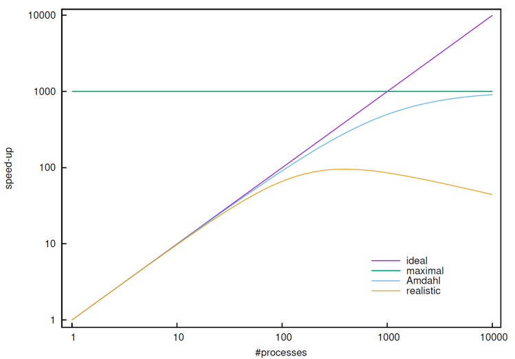
For the curve named “realistic” it is additionally considered that overheads for communication and synchronization will also increase when the number of processes is increased. It is immediately apparent that speedups above \(100\) are hardly achieved in practice, even if the parallelizable part of a program is \(99.9\%\).